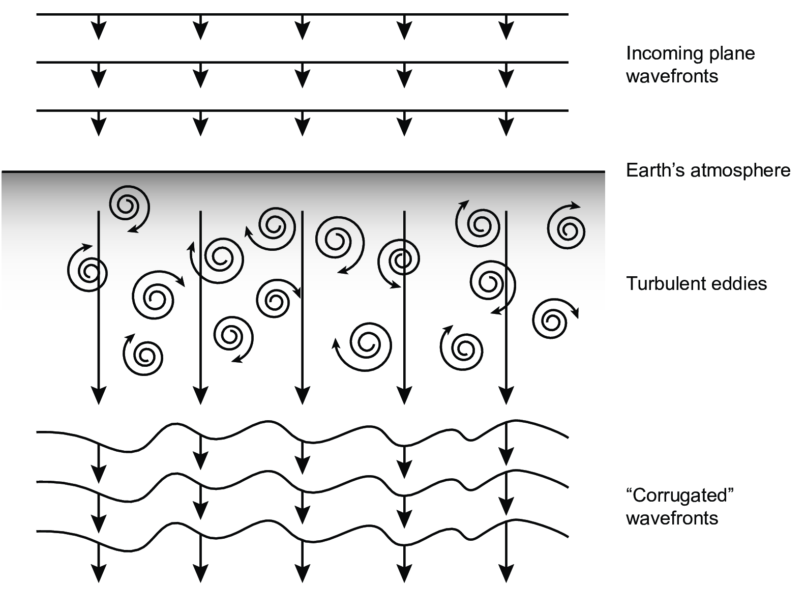Figure 3.1: Schematic diagram of an initially-plane wavefront propagating through the atmosphere. SVG file: corrugated-waves.svg

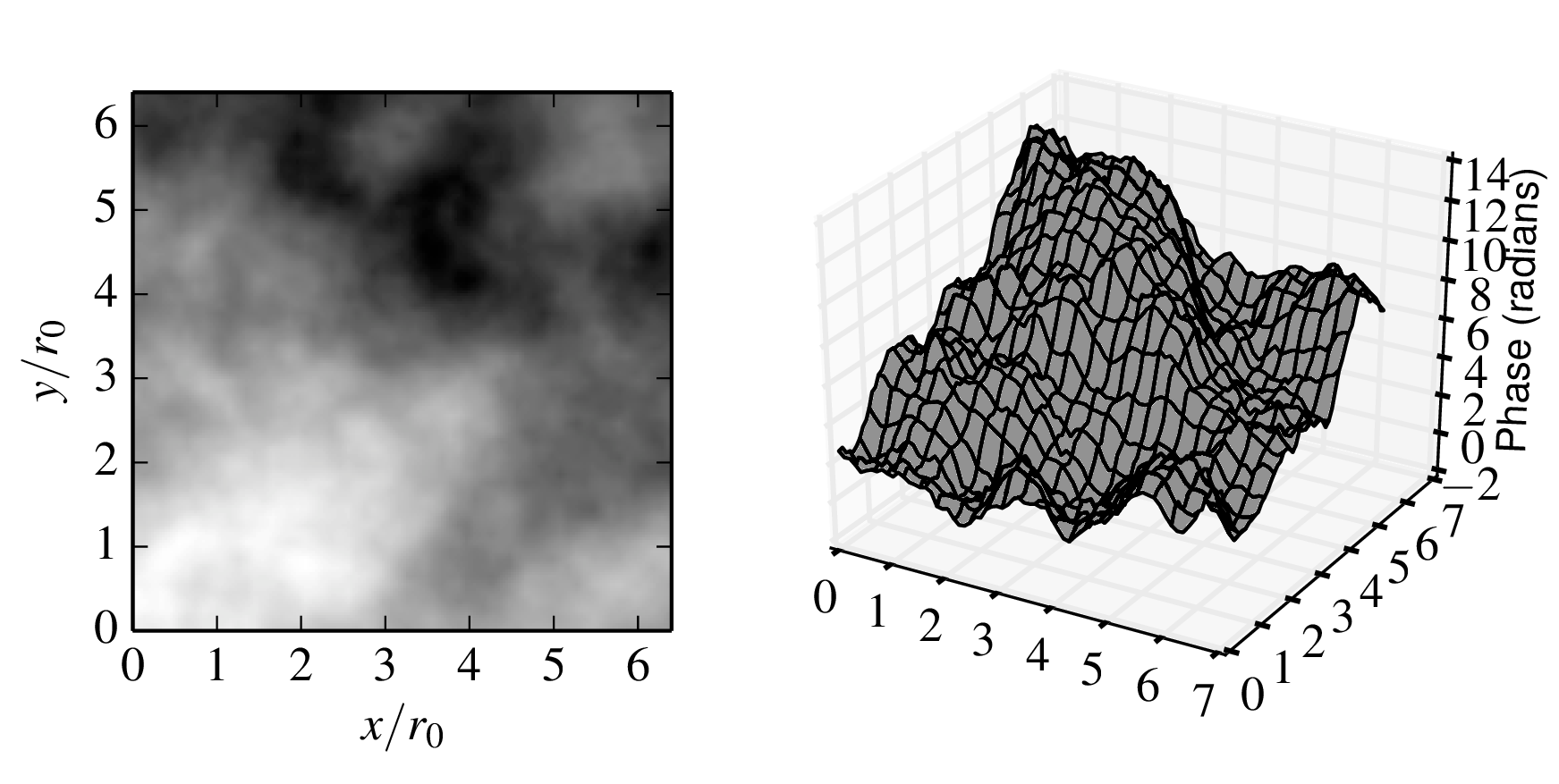Figure 3.2: Atmospheric wavefront perturbations generated using a numerical simulation. The left hand image is a greyscale image of the surface plotted on the right. Python file: phasescreen.py

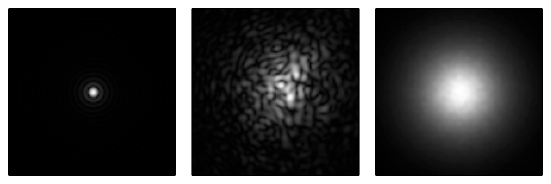Figure 3.3: Simulated images of a point source of light (a) seen through a diffraction-limited telescope of diameter d (b) seen in a short exposure through the same telescope affected by atmospheric seeing with a Fried parameter given by r₀=0.1d and (c) seen in a long exposure through the same telescope and seeing. Python file: speckle.py

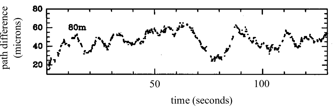Figure 3.4: The motion of fringes seen on an 80-metre baseline on the SUSI interferometer. From . SVG file: davistemporal.svg

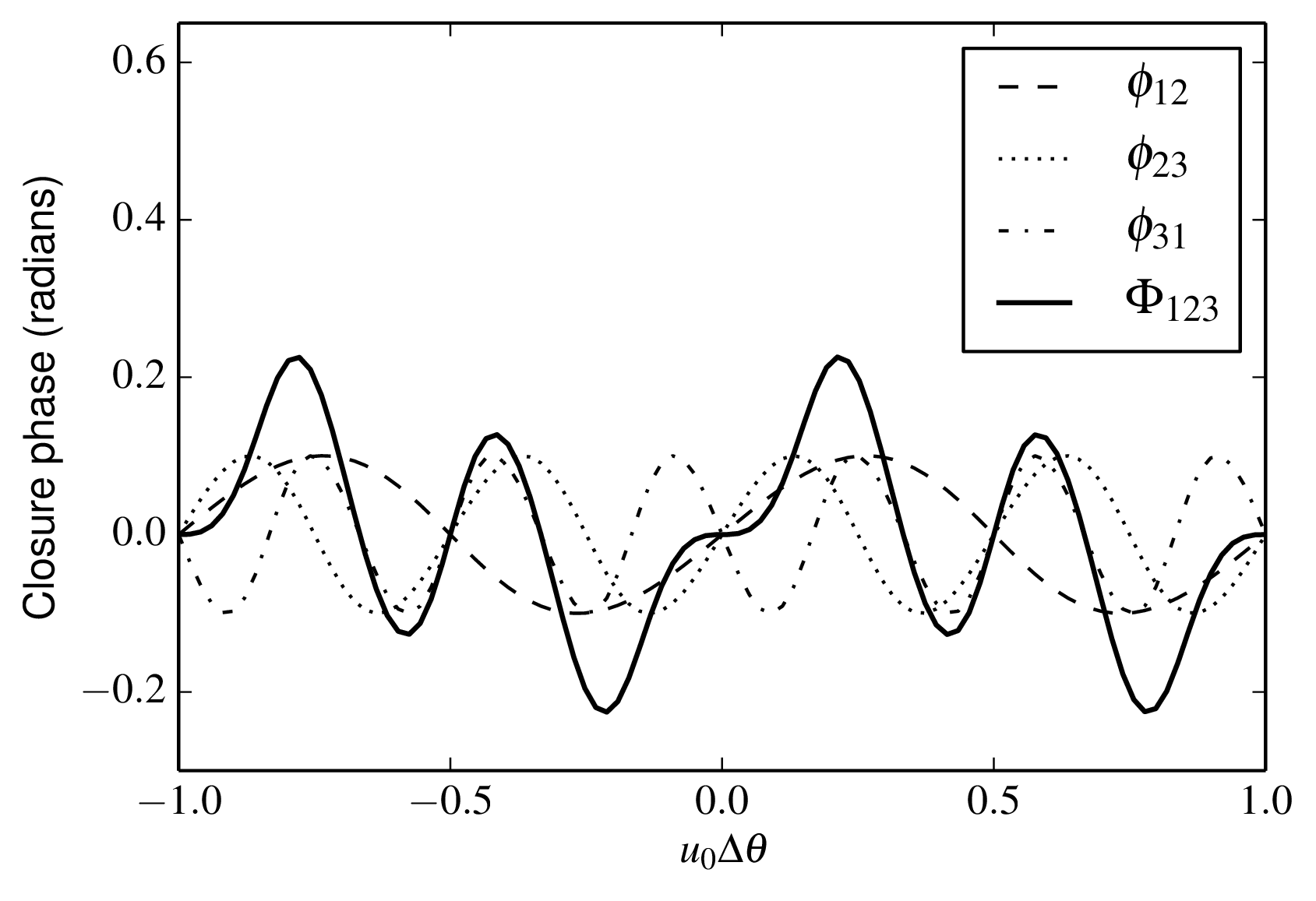Figure 3.5: The closure phase measured on a binary star system as a function of the separation ∆θ of the pair of stars. The flux ratio of the pair is 10:1. In this one-dimensional example, the baselines form a "linear triangle" with lengths u₀, 2u₀ and 3u₀ and the angular separation of the pair of stars is assumed to be parallel to the direction of the baselines. The individual phases ϕ₁₂, ϕ₂₃ and ϕ₃₁ are shown, together with the closure phase ϕ₁₂₃=ϕ₁₂+ϕ₂₃+ϕ₃₁. Python file: clpbinary.py

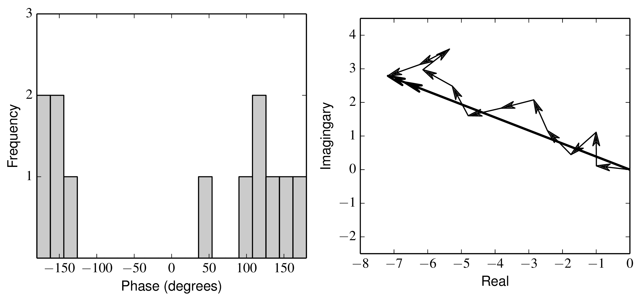Figure 3.6: Histogram of a sample set of phases (left) and "vector averaging" of this set of phases (right). The arithmetic average of the phases is 3^° , while the vector average phase is 159^° . Python file: vectoraverage.py

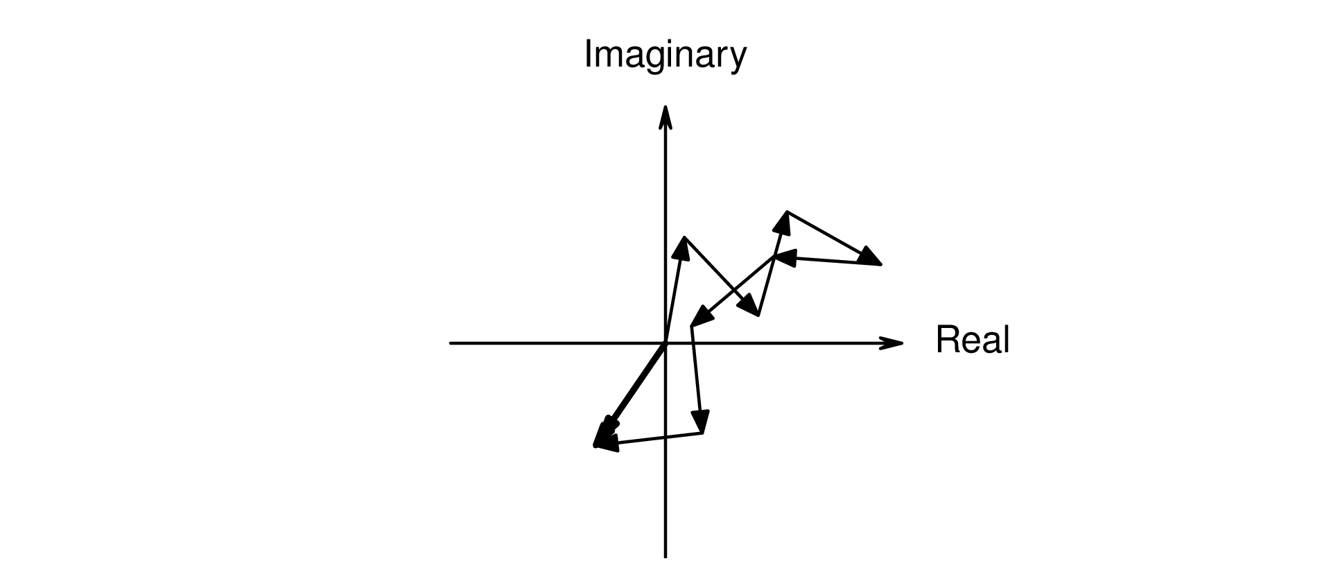Figure 3.7: A simple random-walk model for the fringe visibility. Python file: randomwalk.py

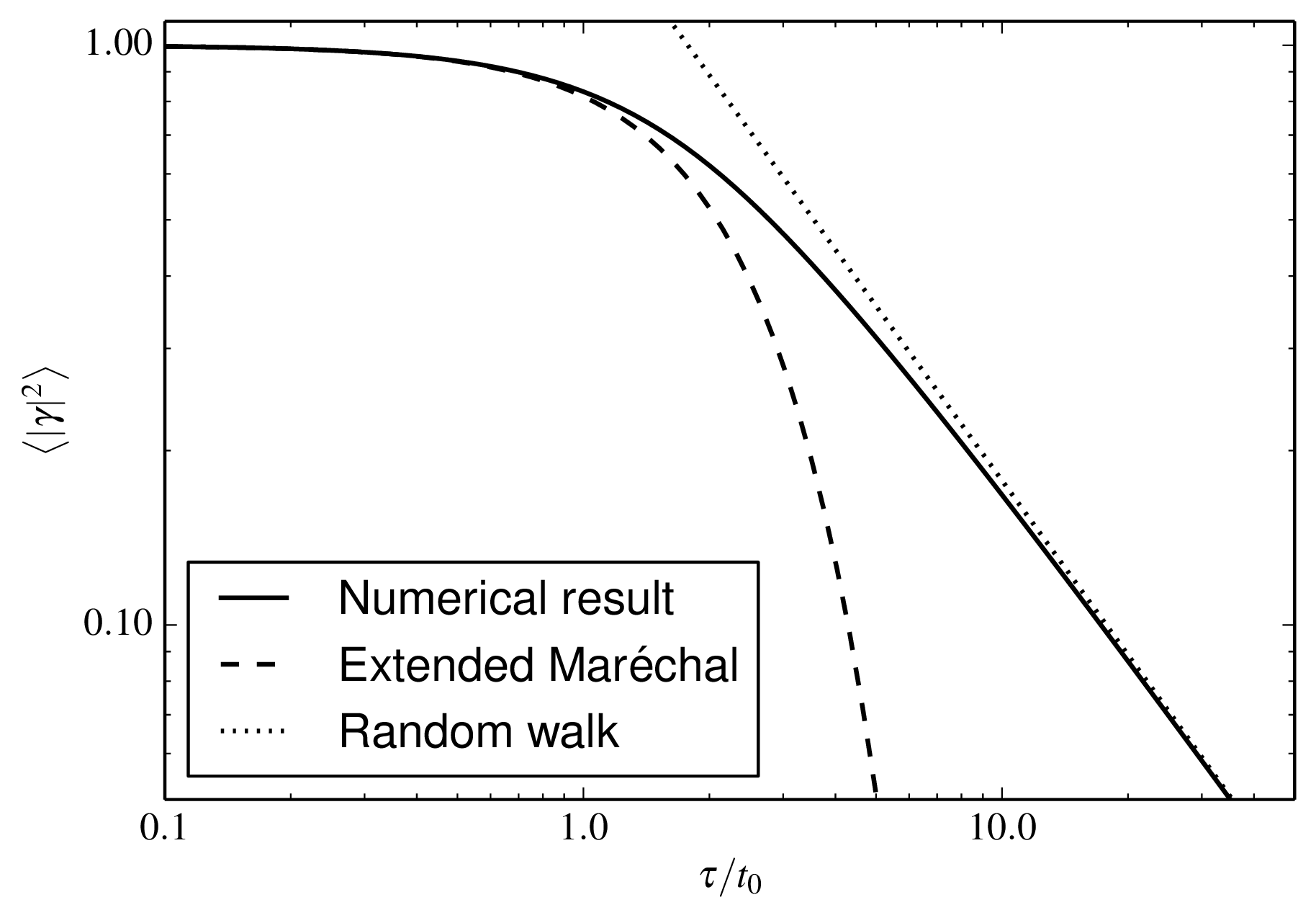Figure 3.8: The mean squared visibility loss 〈 |γ|² 〉 as a function of exposure time τ. Also shown are approximate expressions for large and small τ. Python file: vistime.py

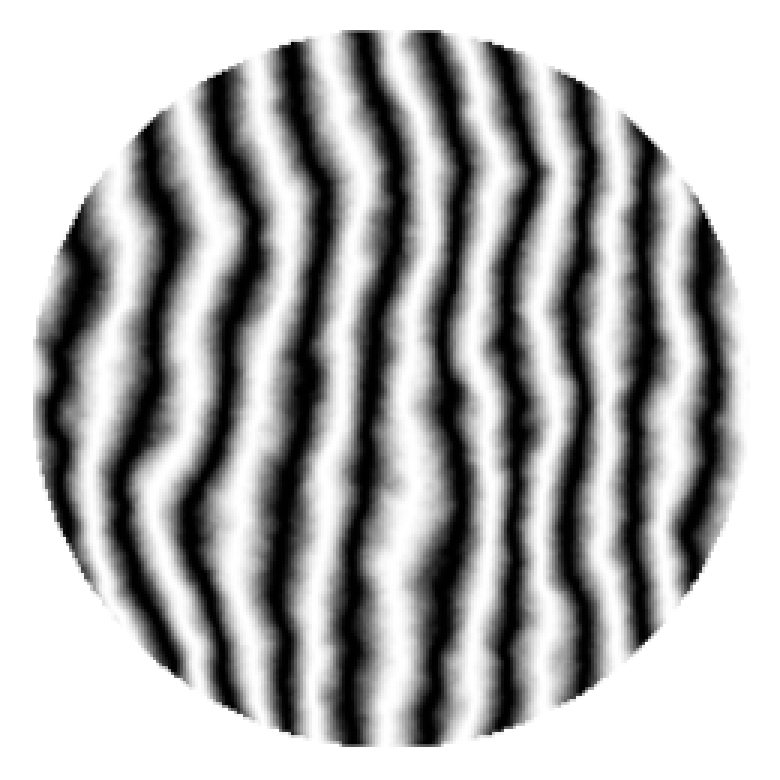Figure 3.9: A simulated pupil-plane fringe pattern in the presence of atmospheric phase perturbations. Python file: fringedistortions.py

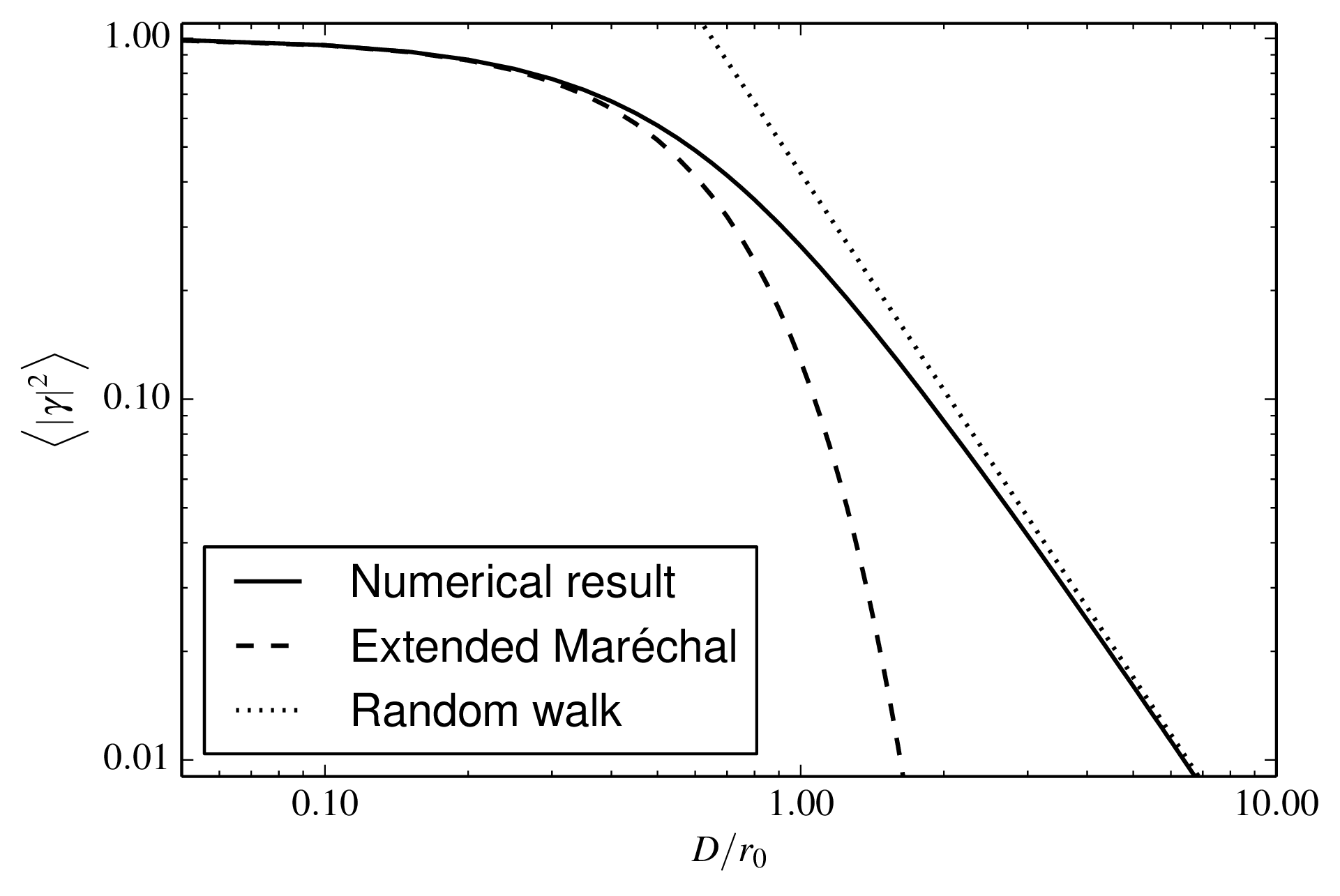Figure 3.10: The mean squared fringe visibility loss 〈 | γ|² 〉 as a function of aperture diameter D for a pair of well-separated circular apertures in Kolmogorov turbulence. Also shown are approximate forms for 〈 | γ|²〉 when D << r₀ and D >> r₀ Python file: uncorrected.py

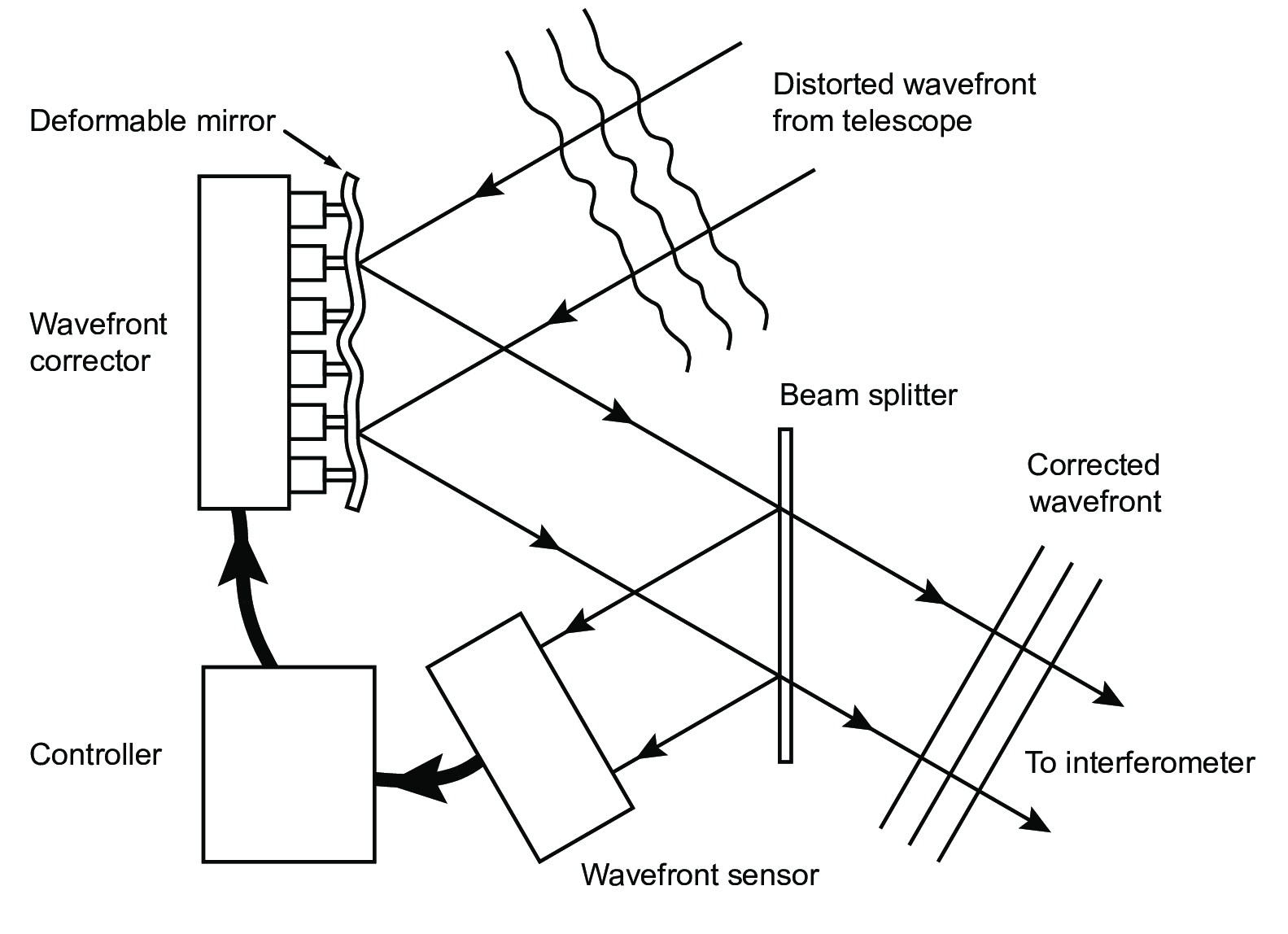Figure 3.11: Schematic diagram of an adaptive optics system on a telescope SVG file: AO.svg

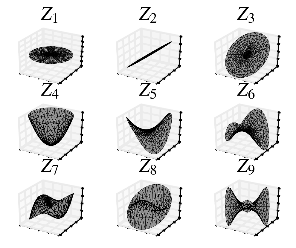Figure 3.12: Surface plots of the lowest order Zernike polynomials. Python file: zernikesurface.py

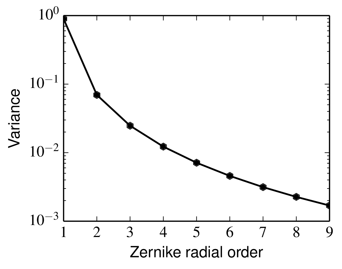Figure 3.13: The variance of the coefficients of the Zernike modes in the wavefront perturbations produced by Kolmogorov turbulence. The variances for all modes with the same radial order are the same []; what is plotted is the total wavefront variance contributed by all n+1 modes corresponding to a given radial order n. The variance is plotted for an aperture diameter of D/r₀=1 and scales as ( D/r₀ )^5/3. Python file: nollvariance.py

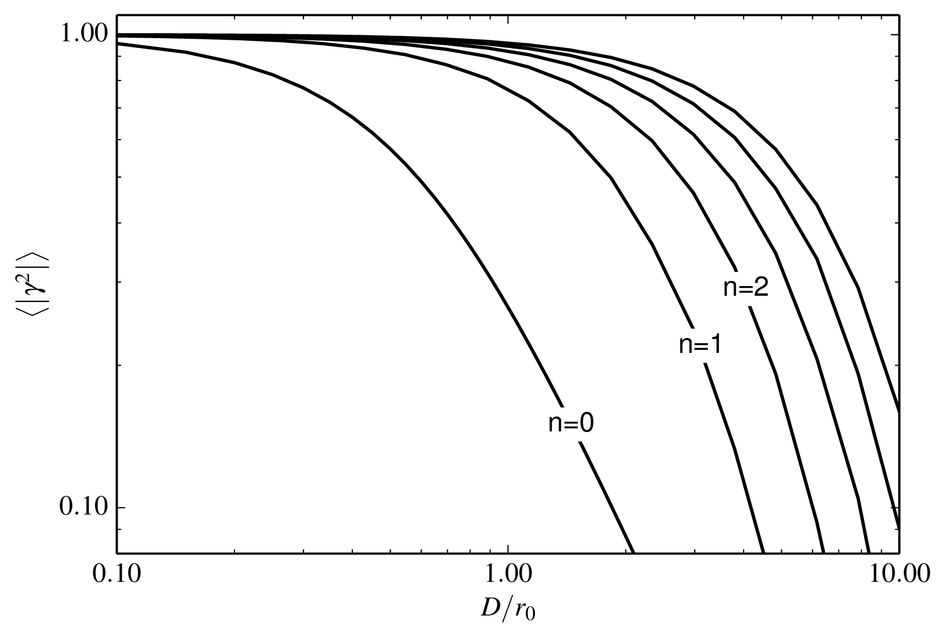Figure 3.14: The mean squared visibility loss 〈 |γ|² 〉 as a function of aperture diameter D for an interferometer with an AO system at each telescope. AO systems which remove increasing numbers of low-order wavefront modes are shown and are labelled by the maximum Zernike radial order n corrected. An interfermeter with no correction (n=0) is also shown for comparison. Python file: aovisibility.py

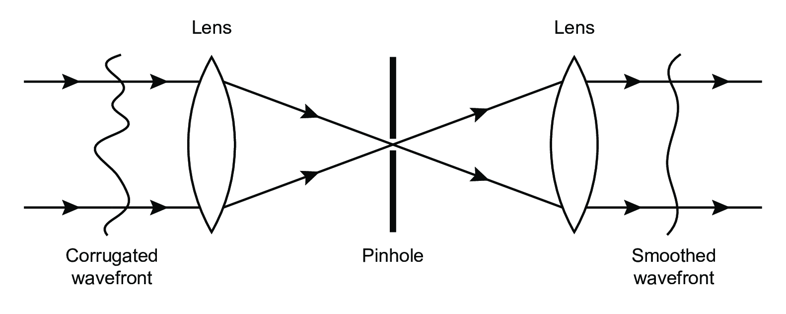Figure 3.15: Layout of a spatial filtering arrangement using a pinhole. SVG file: pinhole.svg

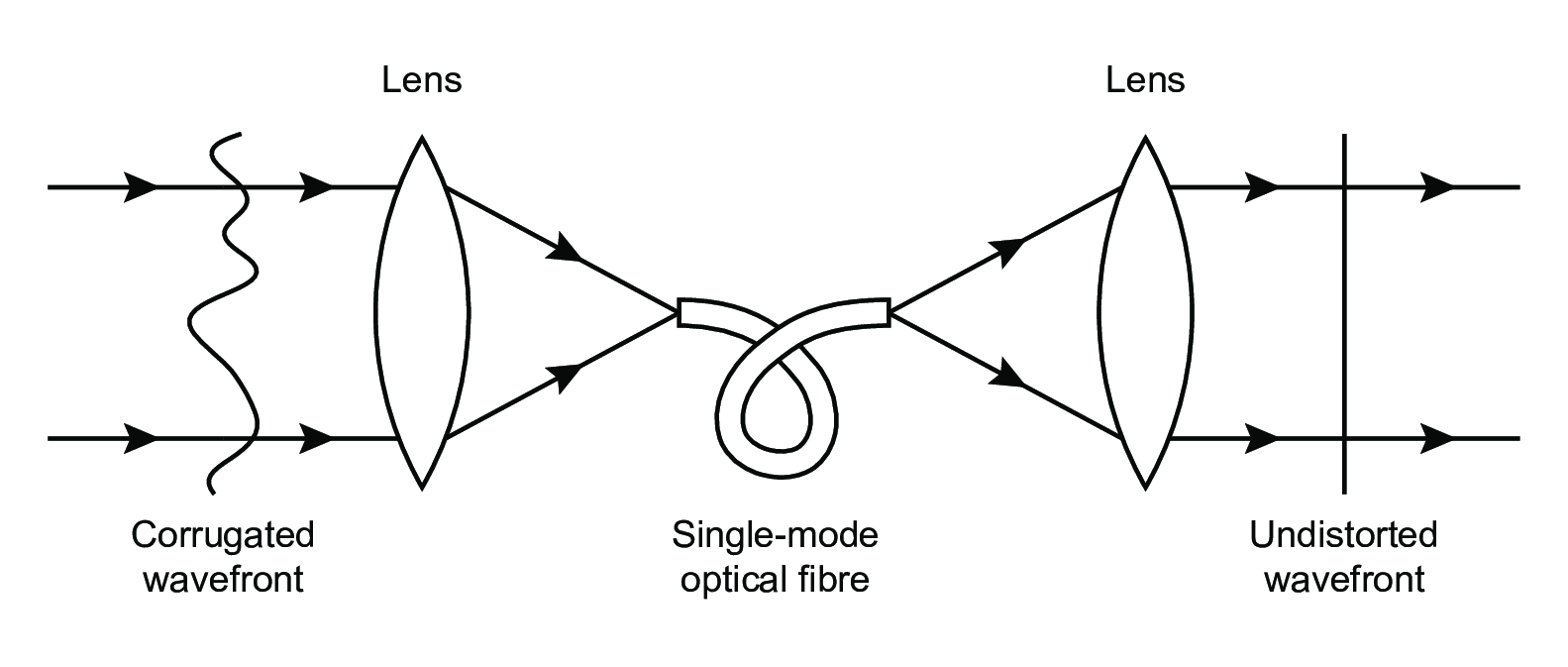Figure 3.16: Layout of a spatial filtering arrangement using a single-mode optical fibre. SVG file: monomode.svg

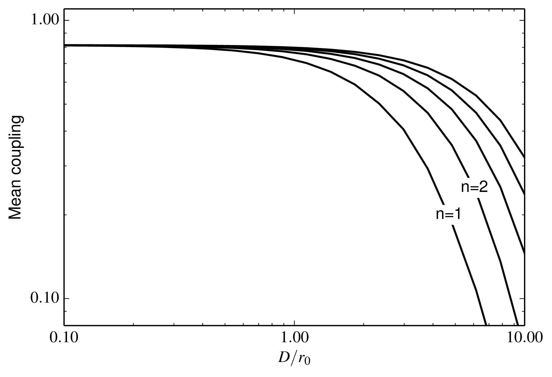Figure 3.17: Fraction of starlight coupling into a single-mode fibre spatial filter as a function of the size of telescope for different levels of adaptive correction. The maximum Zernike radial order n removed by the adaptive optics system is indicated for each graph. The fibre mode is assumed to have a far-field pattern which is Gaussian in shape and has a 1/e radius which is 0.9 times the radius of the beam from the telescope: this choice gives approximately optimal coupling. Python file: aofiber.py

Figure 3.18: Example layout for an interferometer with a separate fringe-tracking beam combiner and science beam combiner. SVG file: fringe-tracker-science.svg