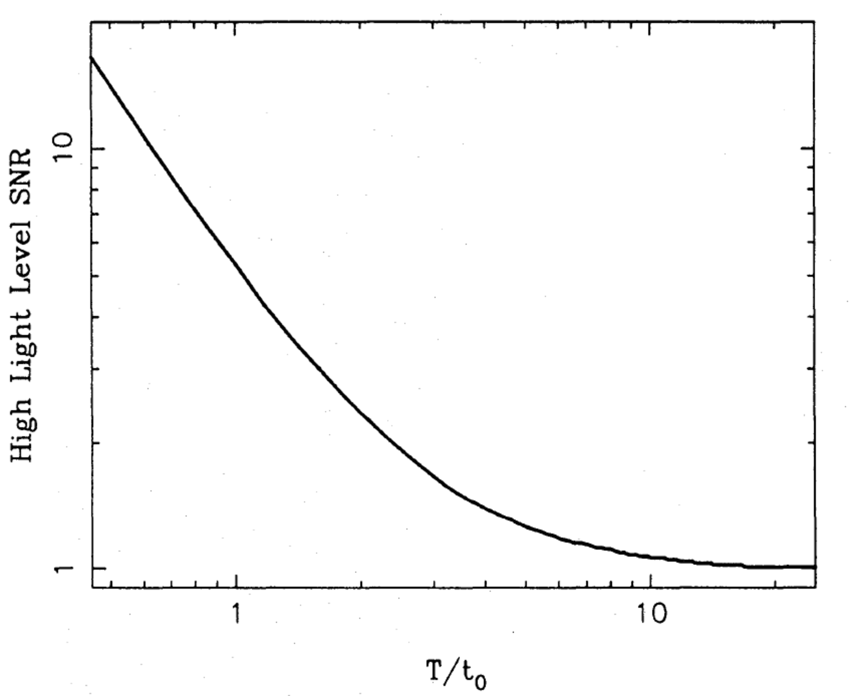Figure 5.1: The SNR of atmospheric-noise-limited measurements of fringe amplitude as a function of exposure time. The SNR is defined as the mean squared visibility modulus divided by the standard deviation of the squared modulus. From .

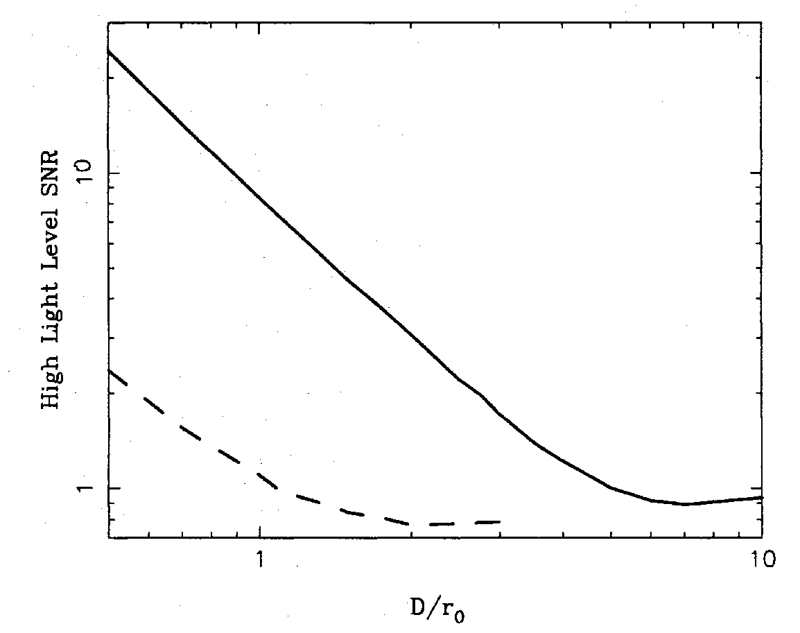Figure 5.2: signal-to-noise ratio for atmospheric-noise-limited observations through apertures of different diameters (from ). The solid line corresponds to a tip-tilt corrected aperture and the dashed line to an uncorrected aperture.

Figure 5.3: Sample bispectrum values plotted on an Argand diagram. The values were measured using aperture masking on a bright point source (α Boo) with sub-r₀ subapertures. The scatter is larger in the direction parallel to the mean bispectrum value than in the perpendicular direction, suggesting that the exposure time used was much greater than t₀. From

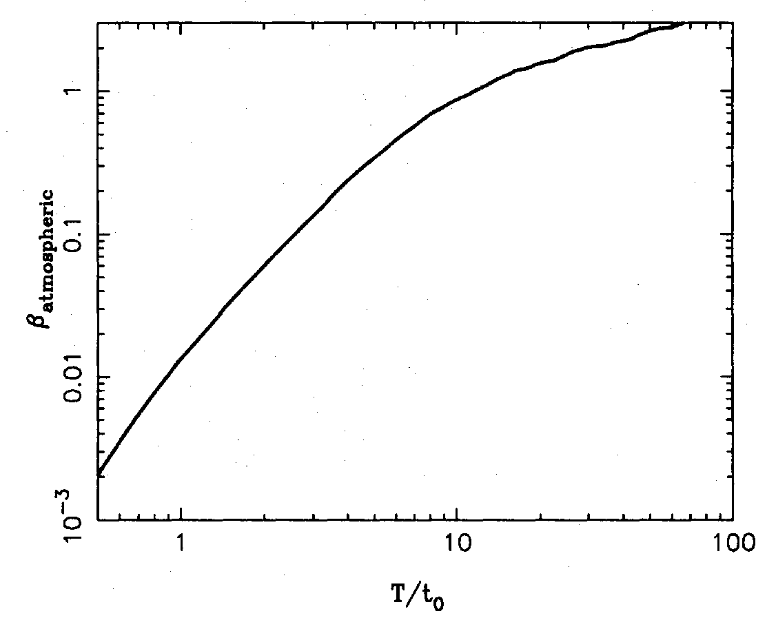Figure 5.4: The phase error σ_ϕ on the bispectrum as a function of exposure time for atmospheric-noise-limited measurements. From .

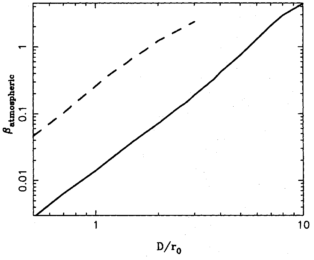Figure 5.5: The phase error σ_ϕ on the bispectrum as a function of aperture diameter for atmospheric-noise-limited measurements. The dashed line is for no adaptive optics correction and the solid line is for tip-tilt correction. From .

Figure 5.6: The signal-processing chain for a single pixel of a photoelectric detector. Light enters as photons on the left and exits as a digitised electrical signal on the right. ADC stands for analogue-to-digital converter. SVG file: pixel-signal-chain.svg

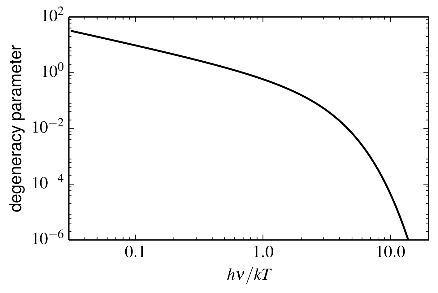Figure 5.7: The photon degeneracy parameter (photons per unit frequency per unit time in a single spatial mode) for thermal radiation at frequency ν from a black body at temperature T. Python file: degeneracyparameter.py

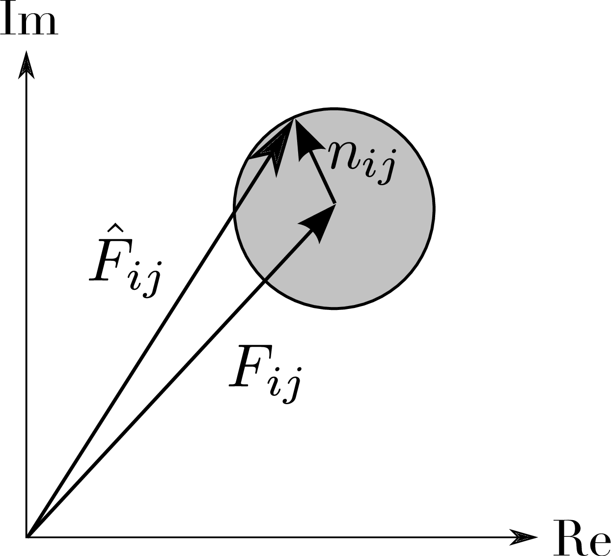Figure 5.8: Argand diagram representation of the estimator ∧F_ij for the fringe coherent flux as a sum of the true coherent flux F_ij and the complex noise n_ij. It can be seen that the complex noise gives rise to both amplitude and phase errors in the estimate. SVG file: noise-vector.svg

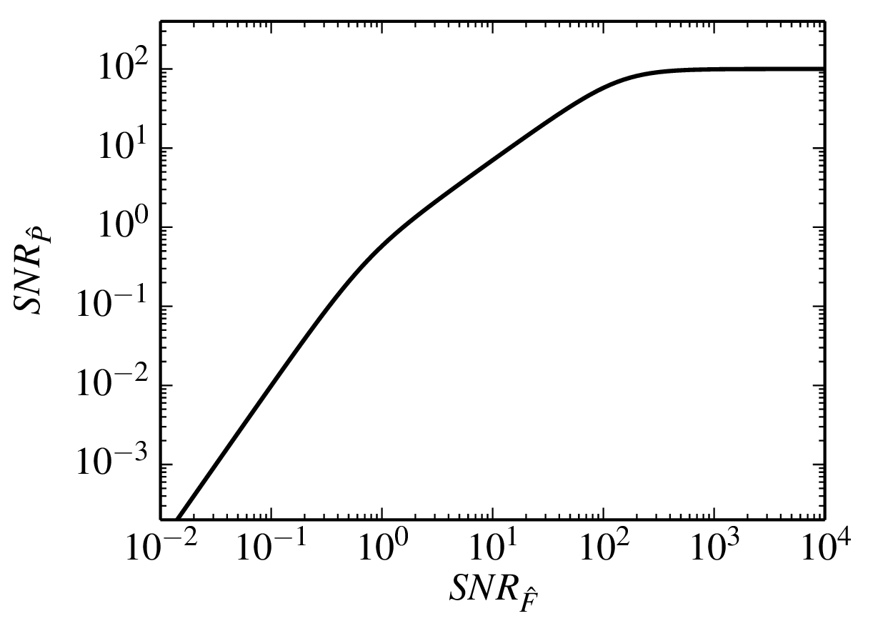Figure 5.9: The signal-to-noise ratio of the power spectrum as a function of the signal-to-noise ratio of the coherent flux. The atmospheric-noise-dominated signal-to-noise ratio has been assumed to be of order 100. Python file: powerspectrum-scaling.py

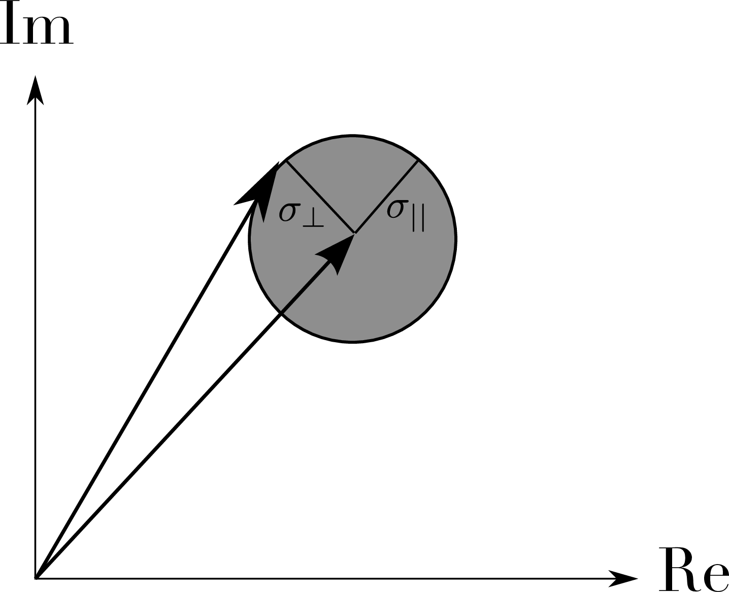Figure 5.10: Schematic diagram of the noise on the bispectrum. SVG file: bispectrum-noise.svg